BAD Day 1: One way ANOVA

This notebook is intended to demonstrate the application of the one way ANOVA analysis on a built in R data set: PlantGrowth

In [1]:

# Getting the data set and having a peek into its content
help(PlantGrowth)
PlantGrowth

weight	group
4.17	ctrl
5.58	ctrl
5.18	ctrl
6.11	ctrl
4.50	ctrl
4.61	ctrl
5.17	ctrl
4.53	ctrl
5.33	ctrl
5.14	ctrl
4.81	trt1
4.17	trt1
4.41	trt1
3.59	trt1
5.87	trt1
3.83	trt1
6.03	trt1
4.89	trt1
4.32	trt1
4.69	trt1
6.31	trt2
5.12	trt2
5.54	trt2
5.50	trt2
5.37	trt2
5.29	trt2
4.92	trt2
6.15	trt2
5.80	trt2
5.26	trt2

We will now use the summary functon to get more information about the whole data set

In [2]:

# Getting a basic summary of the data
summary(PlantGrowth)

     weight       group   
 Min.   :3.590   ctrl:10  
 1st Qu.:4.550   trt1:10  
 Median :5.155   trt2:10  
 Mean   :5.073            
 3rd Qu.:5.530            
 Max.   :6.310

You can also get statistical information on a single attribute of the data

In [3]:

# Computing the SD of a given attribute
sd(PlantGrowth$weight)

0.701191842508168

Or per groups within the data set

In [4]:

# Compute the sd of each group for the given attribute
tapply(PlantGrowth$weight, PlantGrowth$group, sd)

ctrl: 0.583091378392406
trt1: 0.793675696434703
trt2: 0.442573283322786

The next thing we will do is creating a boxplot of the data set (as in the main Tutorial).

In [9]:

boxplot(weight ~ group, data =  PlantGrowth, col = 'mediumpurple',
        xlab = 'Group', ylab = 'Weight')

png

We can also create histograms of the data. In this case we will use the lattice plotting system:

In [10]:

# Creating a conditional histogram of the data
par(mfrow =  c(1,3))

# We will use the lattice plotting system
library(lattice)

# Creating the histogram
histogram(~weight | group, data =  PlantGrowth, col = 'mediumpurple', type = 'count')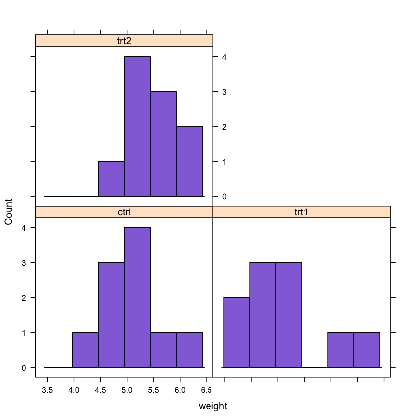

png

** Our null hypotesis is that the three groups have the same growth mean**

First we will use a completely randomized design one-way ANOVA

In [14]:

# One way ANOVA (Randomized design)
analysis <- aov(weight ~ group, data = PlantGrowth)
summary(analysis)

            Df Sum Sq Mean Sq F value Pr(>F)  
group        2  3.766  1.8832   4.846 0.0159 *
Residuals   27 10.492  0.3886                 
---
Signif. codes:  0 ‘***’ 0.001 ‘**’ 0.01 ‘*’ 0.05 ‘.’ 0.1 ‘ ’ 1

Now we will build a linear model with lm() and will then use the anova() command to analyse the fit

In [12]:

fit <- lm(weight ~ group, data = PlantGrowth)
anova(fit)

	Df	Sum Sq	Mean Sq	F value	Pr(>F)
group	2	3.76634	1.8831700	4.846088	0.01590996
Residuals	27	10.49209	0.3885959	NA	NA

As expected, both approaches provide the same results!